What Survival Buys
Continual learning as what an agent has to do to keep existing on a budget — retention as plasticity control rather than caching, the price of being easy to update, and several ways to write the problem down
Research note
The frame
An agent lives in an environment. It acts, and the environment answers with feedback — outcomes, costs, and consequences that depend on what it did. It runs on a budget: time, energy, memory and computation, each finite, each spent by acting, and not freely interchangeable with the others. Failure is absorbing: there is a floor below which the agent cannot continue and from which it does not return. And its goals, whatever they are, are conditional on being alive to pursue them.
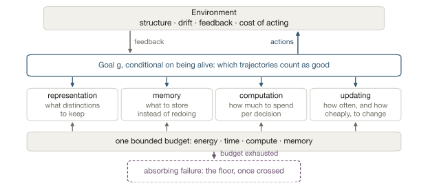
That is not a theory. It is the situation of anything that has to keep running. What is open is what follows from it — and one consequence is easy to skip: the horizon is not a parameter of the problem. An agent that survives longer gets more chances to act, so how long it has is an output of its own decisions, not a number handed to it.
One caveat belongs up front, because it limits what the frame can be used for. Bounded resources alone do not imply that learning must continue. A stationary, fully observed decision process admits a stationary optimal policy [21], and an agent that has found one has nothing left to learn — the second half is an inference, not a theorem in that book. What forces continued adaptation is the combination of limited resources with an environment that does not hold still: partial observability, drift, and the informational capacity a finite budget buys. That argument has been made precisely, as reinforcement learning under a computational constraint [10], including the result that even in a stationary environment an informational constraint can make perpetual adaptation worthwhile, and a companion treatment of allocating capacity across sub-problems [11]. Anything below that sounds like “bounded resources make learning necessary” should be read against that.
Four decisions run through it: what survival makes of the objective, of memory, of representation, and of the agent’s own willingness to change. What the note adds, stated here rather than saved for the end, is a reading rather than a theorem: the horizon is an output of survival, the lower tail is what the retention and update decisions are priced against, and retention, representation and the cost of changing are one frontier seen from three sides — argued with five formulations, four small simulations, and nothing proved.
Five formulations, and what each hides
Everything in this note is a model, and a model is not the thing. Each of the following is a way of writing the same situation down; each makes some questions easy and others invisible. None of them is the problem. The point of saying this here is that the choice should be deliberate, and its cost should be visible on the page rather than hidden behind an equation.
Maximum average reward subject to a compute budget. Posit an objective to be maximised over an indefinite lifetime and a constraint on the compute available to maximise it ([10] formalises it as parameters times gradient steps). This is the natural home for the trade-offs the field already names: information capacity follows from compute, regret provably persists, and adaptation can pay even when nothing changes [10] [11]. What it does not contain is death. A constraint on compute is a tax; a floor is a boundary.
The probability of persisting to a horizon. Ask instead how often the agent is still alive at time \(T\). That is exactly an undiscounted indicator-reward problem, with a stationary optimal policy [40]. It is the cleanest formulation of survival, and its limitation is the mirror image of the previous one: it ranks nothing among the survivors. A policy that scrapes along indefinitely and one that flourishes indefinitely can score identically.
A multiplicative cost functional. Write the value of a lifetime as the expected product of per-step factors, \(\mathbb{E}\left[\prod_t c(x_t,u_t)\right]\). This is the classical home of the observation that accumulation over an open horizon is multiplicative rather than additive [41]. Its practical surrogate — a per-step reward equal to the logarithm of the survival probability — is a known lower bound on the true objective rather than an identity [42]. That gap is why the survival numbers below are simulation results and not a theorem about optimal policies.
A viability constraint. In viability theory the question is not what to maximise but which trajectories are admissible: survival is a set the agent must stay inside, with no cost functional at all [36]. This buys the sharpest available statement of “death is not a penalty to be traded against reward”. It says nothing about what to do while staying inside the set, which is the rest of the problem.
An allocation over \(k\) budgets. Treat the agent as allocating time, energy, memory and compute under constraints, with the achievable set a frontier rather than a single optimum [6] [16]. This is the formulation used for the resource half of this note, and it inherits the weakness of all allocation models: it takes the objective as given, when the interesting part is often that the objective is what the agent is trying to discover.
So: five partial models, each wrong in a specific way, each useful for a specific question. The rest of this note uses the persistence formulation to reason about survival, the multiplicative one to reason about growth, and the allocation one to reason about resources — and where a claim depends on the formulation rather than on the world, it says so.
Survival is decided by the tail
Everything quantitative below comes from four small simulations of the models in this section and the two that follow. The equations are exact for the models they describe and the models are partial; three caveats run through the argument and each is stated where it bites. Accumulation is assumed multiplicative. The log surrogate for survival is a lower bound, not an identity. And the effect has force only when the aggressive policy has negative log-growth or a total-loss tail.
The smallest model that bites
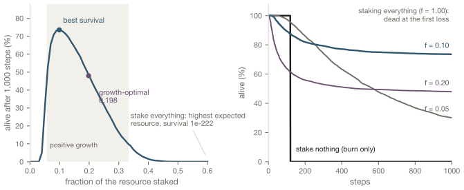
The mean and the tail disagree in the smallest model that has both, and the mean is the criterion that selects the policy which cannot survive. An agent holds a resource that decays by 1% per step whatever it does — the price of existing. Each step it stakes a fixed amount \(f\) — measured in units of the starting resource, not a fraction of what remains — on an even-money bet it wins with probability 0.6. There is a floor at 30% of the starting resource: below it, the agent stops.
Three criteria, applied to the same family of policies, disagree.
- Expected wealth asks how large the resource is on average. It is largest when the agent stakes everything. At \(f = 1\) the multiplier is 1.99 on a win and \(-0.01\) on a loss, so it averages \(0.6 \times 1.99 - 0.4 \times 0.01 = 1.19\) per step (decay included), and expected wealth after a thousand steps is about \(3 \times 10^{75}\). Nearly all of it rides on the single path where every bet wins, an event with probability \(1.4 \times 10^{-222}\). The average is a number no trajectory can expect to see.
- Growth asks at what rate the resource compounds in the typical case, which is the average of the logarithm of the per-step multiplier. It peaks at \(f = 0.198\), the classical growth-optimal criterion [1].
- Survival asks how often the agent is still above the floor. Over the same 1,000 steps it is highest near \(f = 0.10\), where 74% of 4,000 simulated agents are still alive.
The three criteria select three different policies.
The band of stakes at which the resource compounds upward at all runs from 0.058 to 0.332, and its two edges fail for different reasons. Below the band, a stake too small earns less than the 1% burn costs: an agent that stakes nothing crosses the floor after about 120 steps, since the burn alone gives \(0.99^{120} \approx 0.30\), and survives 0% of episodes. Above the band, losses compound faster than wins repair them, so the average of the logarithm turns negative even though the average multiplier is still above 1. In a system that has to pay to exist, inaction is also a way to die.
Why survival is not growth
The shape of that curve follows from a classical result rather than from the simulation. Write \(M\) for the per-step multiplier, \(g = \mathbb{E}[\log M]\) for its log-growth, and — where \(g > 0\) — let \(\theta > 0\) be the positive root of \(\mathbb{E}[M^{-\theta}] = 1\), the adjustment coefficient of the log-wealth walk, standard in ruin theory. With the floor at log distance \(a = \log(1/0.30) = 1.204\) below the starting resource,
\[ \begin{aligned} \Pr(\text{ruin}) \;&=\; 1, && g \le 0, \\[2pt] \Pr(\text{ruin}) \;&\le\; e^{-\theta a}, && g > 0 . \end{aligned} \]
So persistence needs positive log-growth, and even then the ruin probability falls with the mean of log returns and rises with their spread. The second line is the classical Lundberg bound [29], and it is a bound rather than an identity. For \(g > 0\) the exact statement is
\[ \Pr(\text{ruin}) \;=\; \frac{e^{-\theta a}}{\mathbb{E}\left[\,e^{\theta O} \mid \text{ruin}\,\right]} , \]
where \(O \ge 0\) is the overshoot: how far below the floor the walk lies when it first crosses it. The denominator is 1 exactly when the crossing lands on the floor and greater than 1 whenever a step carries it past, so the bound overstates ruin — the true probability is strictly smaller unless every ruin path lands exactly on the floor. That is part of why the simulated survival below sits above what the bound guarantees; the rest is the finite horizon. Deepen the floor and the excess settles into a constant, \(\Pr(\text{ruin}) \approx C\,e^{-\theta a}\) with \(C \le 1\) — the Cramér–Lundberg approximation. Where the log-increments are roughly normal, \(\theta \approx 2g/v\) and the bound is approximately \(e^{-2ga/v}\) — the variance sitting in the exponent. That substitution approximates the exponent rather than supplying a second bound, and it improves as the steps get small.
The bound locates the optimum rather than merely describing it. At \(f = 0.10\) it puts the eventual survival probability at no less than 70.7%, against the 73.6% still alive at 1,000 steps; at the growth-optimal \(f = 0.198\) it puts it at no less than 45.6%, against 47.9%. Both simulated numbers are still falling toward the limit, which is what a finite horizon should do. Maximising the survival probability the bound guarantees puts the survival-optimal stake at \(f = 0.099\) — where the simulation’s 0.10 sits — well below the growth-optimal 0.198. The mechanism is that a larger stake buys a higher growth rate and pays for it with a variance that enters the exponent: growth and security are different functionals of the same distribution, and the mean of the multiplier is neither of them.
The mean is not merely a worse summary here. It is the one criterion of the three that picks the policy which cannot survive. Growth-optimal play maximises growth, not security: the probability of staying above a given floor is maximised by a smaller stake, and fractional stakes trace the frontier between the two [27]. That separation is a finite-horizon effect, and it is why gambles are also ranked by the probability of falling below a floor [28].
Two policies, one mean
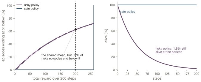
A sharper version needs no betting at all. Take two policies over 200 steps. One collects 1.0 per step and cannot fail. The other collects \(r\) per step while alive and dies with probability 0.02 each step. The expected number of steps alive is \((1 - 0.98^{200})/0.02 = 49.12\), so \(r = 200/49.12 = 4.072\) makes the two undiscounted expected totals equal at 200.0 — and that is the only statistic under which they tie, which is the point: an undiscounted average return over a fixed window, which is what a benchmark reports, cannot tell them apart. Everything about their persistence can. 63% of the risky policy’s episodes end below that shared mean, its median total is 140, its fifth percentile is 8.1, and 1.8% of episodes are still alive at the end. Discount the future at all and the risky policy wins instead, because its reward is front-loaded.
Why the mean and the tail come apart
The mechanism is worth stating exactly, because the honest version of the claim is narrower than the slogan. When value accumulates multiplicatively over surviving steps, the additive quantity is the logarithm, and \(\mathbb{E}[\log W] \le \log \mathbb{E}[W]\), with equality only for a certain outcome. This is where time averages and ensemble averages come apart [2]. Over an indefinite horizon, the probability of still being alive at time \(T\) decays at a rate set by that log-growth, so what decides persistence is the distribution of step outcomes — its lower tail in particular — rather than its average.
Two qualifications. The multiplicativity is an assumption, not a theorem: the logarithm is the ergodic observable for purely multiplicative dynamics and the arithmetic mean for purely additive ones [30], and the process here is multiplicative by construction. And persistence is not a discounted expected-return problem: with a finite discount, the return-maximising policy can have no chance of surviving indefinitely. Its exact homes are the undiscounted indicator-reward problem [40] and the multiplicative cost functional of stochastic control [41]. Two gaps separate that from what a learner can optimise. Reducing multi-step survival to a per-step log reward gives a quantity proportional to a variational lower bound on it [42]; and the log of an expectation is not the expectation of a log, which is Jensen rather than anyone’s theorem. Both gaps are why the numbers below are simulation results.
What survival does not force
The other survival problem demands the opposite behaviour, and it shows what the argument rests on. Reaching a goal before ruin and persisting are different problems, and they can demand opposite behaviour. Classical gambling analysis gives the cleanest example. A gambler who wants to reach a target before going broke should bet boldly when the game is unfavourable, and timidly when it is favourable [3]. The mechanism is not risk appetite: in a subfair game every bet is a losing proposition, so bold play is optimal because it minimises the number of bets taken at a negative edge, while in a favourable game the opposite holds and many small bets are better. The optimal risk posture is set by the odds and by whether the objective is reaching a target or persisting, not by the fact that failure is final.
So tail-awareness is not a consequence of “survival” as such. It is a consequence of persistence over an open horizon, which is the case that matters for an agent that is supposed to keep running rather than to finish something. The sign of the shift is not fixed either: in agents whose action sequences are forcibly terminated once resources run out, the same survival pressure produces risk-seeking as well as risk-averse behaviour, depending on the environment [31].
An independent implementation
A second implementation reproduces the direction exactly, on a different bet: 45% gains of the whole stake, 45% losses of half the stake, 10% losses of the whole stake, with ruin at 1% of the starting resource. Its growth-optimal fraction is exactly one fifth, and survival to 500 steps is 0.9928 there, against \(3 \times 10^{-24}\) at the expected-wealth fraction of one. Exact expected wealth is \(3.8 \times 10^{25}\) at the expected-wealth fraction and \(2.3 \times 10^{5}\) at the growth-optimal one.
Two things belong with that number. The mean is not merely unhelpful there, it is unestimable by sampling: with ruin probability \(10^{-24}\) no simulated episode survives, so the sample mean ranks the wealth-maximiser last and the exact mean ranks it first. And the argument has bite only when the aggressive policy has negative log-growth or a total-loss tail — under a mild 1% edge the same comparison is technically true and practically empty, differing in the fifth decimal place after 500 steps.
Goals are conditional on being alive
Everything so far is about how long a goal can be pursued. The goal itself changes when survival is final, and that is where the frame becomes goal-conditional rather than merely survivalist.
Start with a modelling choice, because it is one and not a consequence of survival. The note takes a goal that is conditional on being alive to leave histories containing death unranked: “how much did it accumulate before dying” has no place in the ordering. That is a stipulation, and a reader is free to make the other choice — a crashed vehicle’s trajectory matters enormously, and “died slowly, having done the work” against “died immediately” is a distinction people price. Given the choice, expected-utility representation over all outcomes is not automatic, and a Markov reward need not exist at all [8]; expressing the goal exactly then takes a history-dependent reward, or a state augmented with the information survival depends on [9]. The non-existence result is a consequence of the modelling choice, not of mortality as such, and saying so is the difference between a stipulation and a derivation.
This is a claim about how the objective must be written down, not about means being wrong. It is also the precise sense in which continual learning is goal-conditional: goals rank the trajectories that are still being lived, and survival decides which of them there are. An agent cannot achieve whatever objective it has been given if it is dead [32], and an agent reasoning about an unfinished goal treats its own continuation as instrumental [33]. Both of those are known results; what the frame adds is that they are not optional details of an objective but the conditions under which any objective is defined.
Learning is bought from the same budget
Learning is not a separate faculty in this frame. It is one of the things the budget pays for: the agent changes what it carries in response to feedback, and every change costs samples, computation, energy, and often some of what it already knew.
What a learning step is
Something in the agent’s state is adjusted so that future behaviour improves on the evidence so far. Whether that is a parameter vector, a table, a program, or a library of reusable parts, the step has a direction and a size, and both are chosen under the budget. The channel that carries the adjustment — the signal from outcomes back to the parts that should change — decides whether the agent learns fast or learns against itself. Three ways of keeping it faithful are known: training with derivative information as well as values [24], matching the backward message a module passes to its neighbours [23], and matching more than a module’s forward output [26].
What a learning step costs
More samples per step cost compute and time; storing what was learned costs memory; maintaining the ability to change costs energy regardless of whether anything is learned [38]. This is the part of the ledger that is easiest to leave implicit and most consequential when the budget is tight: an agent that treats learning as free will spend the whole budget on it and have nothing left to act with.
Why more learning is not better
Updates interfere. Fitting new experience can degrade old competence, and the ability to fit anything at all can decay with use, so that a long-trained system ends up learning no better than a shallow one [22]. Retention and plasticity are both depletable resources, which is why the allocation question — how much to change, how often, and what to protect — is not a question about diligence.
How fast to update
Under drift, the update rate is set by the environment rather than by preference. Tracking a change faster means averaging the noise less, and that trade-off shows up as a variation budget in non-stationary optimisation [45] and as a rate-versus-regret trade under an information constraint [10] [11]. A world that moves faster does not need a better learner; it needs a learner that spends more of its budget on freshness.
Learning changes what there is to learn
Actions determine which states are visited, and therefore which data exist. In control theory this is the dual effect: the action that steers the state also buys the information used to learn about it, so steering and learning separate only when that effect is absent, and are otherwise chosen together [49]. An agent is part of the process that generates its own non-stationarity: what it chooses to do changes the distribution it will later learn from, and when other learners are in the environment, that distribution changes because of them too.
Representations decide what can be learned
A representation is how the agent makes the environment small enough to act on: a map from the history of interaction to something it can compute with. The choice is consequential in both directions, because a representation decides which distinctions learning can see and which differences are collapsed before learning happens.
Adequacy is behavioural
A summary of history is adequate when it can do two things: compute the expected reward the goal defines, and predict what comes next. It also has to be updatable, recursively, from the data the environment supplies. An approximate version of that sufficiency still yields a policy whose loss of optimality is bounded, and such summaries can be learned from data [46]. That is the precise sense in which a representation has to line up with its environment — not a mirror of the environment’s internal structure, but sufficiency for the consequences the goal prices.
Structure is not required
The abstraction classes that preserve optimal behaviour without any condition on the reward are exactly the ones that ignore parts of the environment’s structure, and the guarantee is a per-class error bound rather than a requirement to match the environment [44] [14]. This cuts against the intuition that a better representation is a more faithful one: a representation carrying more structure than the goal needs can make control harder, not easier.
Resolution costs budget
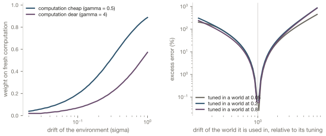
How many distinctions to keep is not free. In the tracking model below, a representation whose timescale is tuned to one world and deployed in another pays 270% more error when the world is eight times slower and 444% when it is eight times faster. The asymmetry is the useful part: the expensive error is being too slow. Adapting faster than necessary wastes computation; adapting more slowly than the world changes is simply wrong, and stays wrong until the world moves again.
What the note is pointing at is the resolution question: non-stationary learning tunes how fast its estimates move — a step size, a restart interval, a variation budget [45] — while the partition that decides how many distinctions exist is usually fixed in advance. Adaptive discretisation is a literature of its own and the search behind this note did not survey it, so the observation is a question rather than a gap.
Memory: keep or recompute
The trade-off, computed
On a budget, remembering and recomputing are alternatives. The alternative to storing a computation is paying to derive it again; the alternative to paying again is not having it when it is needed. Take the simplest tracking problem in which the comparison is exact. A state drifts as a random walk with step size \(\sigma\). The agent’s estimate is an exponentially weighted average of noisy observations, and the weight it places on the newest observation, \(\alpha\), is the dial between trusting what it already has and trusting the sample in front of it. Both ends are failures — \(\alpha \to 0\) lets the estimate freeze while the state walks away, and \(\alpha = 1\) throws away everything but the latest noisy sample — so the optimum is interior. With \(m\) samples per step of variance \(\eta^2\) each, the steady-state error is
\[ \mathbb{E}\big[(\hat{\theta} - \theta)^2\big] \;=\; \frac{\alpha^2\,\eta^2/m \;+\; (1-\alpha)^2\,\sigma^2}{\alpha\,(2-\alpha)} , \]
with retention costing \(\kappa = 1\) per unit of retention, samples \(\gamma\) each, and a total budget of 3, split between the two. A closed form is only as good as the process it describes, so the simulation checks it against the process directly: at \(\sigma = 0.2\), \(\alpha = 0.38\), \(m = 2\), the formula gives 0.1423 and the simulated error is 0.1427.
The allocation then moves as the frame says it should. As drift rises from \(\sigma = 0.05\) to \(0.8\), the optimal weight on fresh computation rises from 0.07 to 0.74 and retention’s share of the budget falls from 31% to 8.6% — holding computation fixed at \(m = 2\) instead of letting the budget re-split gives 0.66 at the top end, so the movement is partly the re-splitting: a world that changes under you is a world in which stored answers expire. Multiply the price of computation by eight and the same agent keeps 29% of its budget in retention instead of 21%. What is remembered is a function of the environment’s drift and of relative prices, and the agent chooses neither.
Why that accounting is not enough
The store-versus-recompute criterion is older than any of this: caching and replacement policies are the same accounting, and they are exactly solvable in the stationary case [12] [13] [47]. What makes it insufficient for continual learning is that the two quantities it compares are not always well defined.
Data that has passed cannot be recomputed at any price, so for much of what an agent retains there is no recomputation alternative to price it against. And when tasks interfere, the value of retaining one item stops being separable from what is retained around it, so per-item prices stop existing. Interference takes two forms: a new update degrades an old capability, and the ability to learn at all decays with use [22]. What is actually stored in that regime is frequently not a cached answer but a constraint: a curvature estimate, a protected subspace, a sample of the past whose purpose is to slow down the wrong kind of change. That distinction is not a footnote to this section — it is a different account of what retention is for, and it is taken up on its own in the next section.
The ingredients for an explicit accounting are published, but they are not joined. Three relevant pieces exist separately. Caching, discarding and recalling samples under a changing context is settled by value of information [43]. The literal store-versus-recompute choice is an old systems problem [47]. And a genuine joint fetch-and-cache cost, minimised over files and time by a learner, exists in network caching [48]. So what is missing is not a per-item price — the paragraph above argues that per-item prices stop existing under interference. It is a system-level accounting: how much capacity to spend on recomputation, on retention, and on protecting retained content from the next update, when drift decides how fast each of those decays. The search behind this note found the pieces published separately and this combination not at all, but the interference objection is why the missing object has to be an allocation rather than a price list.
So retention is an allocation, but the thing being allocated is not one commodity. It buys avoided recomputation where recomputation is possible, protection against interference where it is not, and the option to adapt later.
What a stored computation owes
There is a corollary when what is stored is used inside the loop that keeps learning. A substitute that matches the original’s outputs but not the feedback it passes backward is not a substitute at all: every later update is computed against a different machine than the one the system believes it is running.
Training with derivatives as well as values is an old idea [24], and matching Jacobians between a teacher and a student is an established constraint [26]. The sharpest published version of the local point gives a module both a forward and a backward stand-in, each regressed against its neighbours [23]. Under this frame the point is not exotic: it is the condition on a purchase.
Two kinds of memory, and one prediction
Retention is usually discussed as a storage decision: what is worth keeping, and what should be recomputed instead. That is one half of the problem, and the half the caching literature solves. The other half is not storage at all. What a continual learner keeps is often not a result but a restriction — something whose purpose is to make a future update less damaging.
| cache-like memory | constraint-like memory | |
|---|---|---|
| what is stored | a result: a fused subgraph, a cached embedding, a derived quantity | a restriction: a curvature estimate, a protected subspace, a replay buffer, a trust region |
| what it saves | the cost of deriving the result again | the cost of an update doing damage to what is already known |
| recomputation alternative | exists, and its price is what makes the trade-off | does not exist: the past cannot be re-derived at any price |
| what makes it lose value | drift, which makes stored results stale | a fall in interference: the protection stops being needed |
| how its value is measured | avoided recomputation, minus storage and staleness | avoided loss of old competence, which does not separate item by item |
| the literature | caching and replacement [12] [13] [47] [48] | regularised and projected updates, replay, plasticity maintenance [8] [9] [22] |
The row that matters is the third. A constraint has no recomputation alternative, which is exactly why the caching account does not transfer to it: there is nothing to price it against, and under interference the value of one retained item is not separable from the value of its neighbours. A Fisher matrix, a replay buffer and a frozen subspace are not answers that could have been recomputed; they are commitments about which updates are allowed to happen.
That reframes retention as a plasticity-control decision rather than a storage decision. The question stops being what is worth keeping and becomes how much capacity should be spent gating the next update, and the two are answered by different variables: the storage half by drift and the price of computation, which is what the model in the previous section shows; the control half by how much interference the agent expects between what it is learning now and what it already knows.
Which gives a prediction the storage account does not make, and one that is testable against it. At fixed drift and fixed resource prices, the share of capacity spent on constraint-like retention should rise with interference pressure. The storage account predicts the mix is set by drift and the price of computation alone — the estimator result above is the control, because in it the mixing weight moves exactly with those two and nothing else. So the two accounts are separable by a single experiment.
- Design. Take a continual learner with a fixed budget and a measurable split between stored results and gating structure — the dimension of the protected subspace, the replay allocation, or the fraction of parameters whose updates are constrained. Vary only the interference between tasks: their similarity, or the fraction of shared parameters. Hold the drift rate fixed (task-switch rate, label noise) and hold the memory and compute prices fixed.
- What the storage account predicts. No movement. The mix should depend on drift and prices, both of which are pinned.
- What plasticity control predicts. The constraint share falls as tasks become more similar and rises as they conflict, at constant drift and constant prices.
- What would count against it. Invariance of the mix to interference; or movement that turns out to be interference acting through an effective drift — that is, the only channel by which interference reaches the allocation is the one the storage account already names. Either result would say the two-kind distinction is a description rather than a mechanism.
- Why it is worth running. It is cheap, it needs no new machinery beyond a budget-aware learner that can already protect and store, and its outcome decides which variable a designer should tune: the drift-tracking rate, or the interference rate.
What everything costs
The costs of a learning agent form a ledger, and the ledger has to be written in the currency the agent actually pays. For a decision: latency, energy, memory traffic. For a learning step: samples, computation, and the interference it causes. For retention: storage, maintenance, and staleness. For resolution: the compute that finer distinctions demand at every step.
One rule follows from taking the ledger seriously, and one more follows from the ledger’s shape. Measure what is paid, not what is counted. In the same process geometry, a 32-bit integer addition costs on the order of 0.1 pJ, while a DRAM access costs one to three nanojoules — four orders of magnitude apart [15]. The constraints therefore form a vector, and the achievable set is a frontier rather than an optimum [6]. A proxy like parameter count or nominal sparsity is not a price. The three draws on that budget — recomputation, retention, and protection of what was retained — are the allocation of the memory section, and the price of changing anything at all sets the rate at which the allocation can be revised, which is the subject of the next section.
The ledger is not the only thing the accounting fixes. It also prices the act of changing at all, and that price has a shape worth naming on its own — the next section does it.
Ease of update is worth \(\sqrt{u}\)
Suppose the world moves at a rate \(\delta\) and updating a representation every \(\Delta t\) steps costs \(u\) per update, leaving an error of about \(\delta \Delta t / 2\) as the world drifts away from it. Then
\[ \text{loss} \;=\; \text{floor} \;+\; \frac{\delta \Delta t}{2} \;+\; \frac{u}{\Delta t}, \qquad \Delta t^{*} = \sqrt{2u/\delta}, \qquad \text{loss}^{*} = \text{floor} + \sqrt{2u\delta}. \]
The square root is the result. Being cheap to update is worth \(\sqrt{u}\), not \(u\). A representation that is 25 times cheaper to update is five times cheaper in the error it avoids; making updates four times cheaper again buys only a further factor of two. Investment in updatability has sharply diminishing returns, which is the opposite of what the phrase “make it adaptable” suggests, and it is a closed form rather than a slogan. A rigid representation that fits well at rest (floor 0.05) but costs 0.5 per update loses, above a drift rate of \(\delta^{*} = 0.035\), to a plastic one that fits worse at rest (floor 0.20) and costs 0.02 per update. In a still world the better fit wins; in a moving one the cheaper update wins, and the environment decides which world the agent is in. Note what the threshold is and is not: it depends on the environment’s drift and the two prices, so an agent that declines to invest in adaptability is not being lazy — below \(\delta^{*}\) the investment does not pay, and a learner should be able to compute that from its own budget rather than guess.
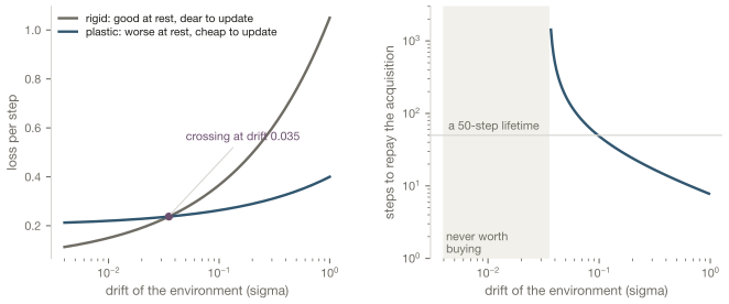
Then the part that looks like recursion and is not. Acquiring the cheap-to-update structure costs something now — say 5.0 once — and repays it over a horizon that falls as the world speeds up: about 173 steps at \(\delta = 0.05\), 24 at \(\delta = 0.2\), and 12 at \(\delta = 0.5\). Below the crossing at \(\delta^{*} = 0.035\) it never repays it, at any horizon. Whether to become easier to change is decided by how long the agent expects to be alive, which is the quantity survival determines and which no single step can see: the cost is immediate and the benefit is not.
The same arithmetic answers when to buy adaptability rather than rent it, and there the horizon enters:
One budget, one allocation
Everything above is one budget with several draws on it. Memory is bought instead of recomputation; resolution is bought instead of approximation error; update frequency is bought instead of staleness; learning itself is bought instead of ignorance. Because the draws compete, the marginal value of each depends on the others. When the terms are separable, choosing them one at a time can still be optimal; the coupling in the retention section is the case where it is not, and there the decisions have to be made together. The arrangement is not unique to machines: allostasis in physiology is the same matching of component capacities to demand, with remembered errors used to reduce future ones [37], and it is an analogy rather than an argument.
Planning with partial information and a bounded memory is hard in the worst case [19], and letting the actions rewrite that memory does not make it easier. The lifetime and absorbing-failure objectives the frame needs form a class of their own, one that needs conditions of its own before it is even well posed [20]. What any agent can do is be bounded-optimal for its machine rather than optimal in the abstract [16].
The object being optimised is the program, for the machine it actually runs on rather than for an abstract ideal [16]; metareasoning then treats the decision of where to spend thought — including spending it early so that later decisions are cheaper — as an ordinary decision [17] [18]. It has a biological form too: maintaining a small labile store that can be changed cheaply, alongside a large stable one, is far more energy-efficient than making every element update in place [38]. Caches of inferences, bought once and reused, are the computational version of the same move [50].
Taken seriously, this puts the agent’s own learning inside its action space. Spending resources now to be cheaper to change later is a normal investment decision: better abstractions, structure that localises an update instead of spreading it, caches of the quantities an update needs. An agent that makes that decision is doing continual learning about its continual learning. That is not a paradox: it is the same allocation problem one level up, and it is the level at which “ease of update” stops being an engineering afterthought and becomes a term in the objective.
The model, assembled
The sections above each solve one decision in its own toy model. This is the schema they are instances of, stated once, with the honest note that a schema is not a solution: only the cells of the table below are solved, and the couplings between them are the open part.
The problem
An agent has an internal state \(z_t\) — its representation, whatever it has retained, and its parameters — and lives in an environment with state \(x_t\). At each step it observes \(y_t\) and takes an action \(a_t\) from a set that includes not only acting on the environment but also choosing how to compute, what to keep, and how to change itself. Every action draws on a budget vector \(b(a_t) \in \mathbb{R}^k\) — energy, time, memory, computation — and lifetime draws are bounded by \(B\). There is a failure set \(\mathcal{F}\): entering it ends the agent, and \(\tau\) is when that happens, whether from a fatal state or from an exhausted budget. A goal \(g\) ranks the trajectories that are still being lived.
The problem is then
\[ \max_{\pi \in \Pi} \;\; \mathbb{E}_\pi\!\left[\sum_{t<\tau} u_g(h_t)\right] \quad \text{subject to} \quad \Pr\nolimits_\pi(\tau > T) \ge 1 - \varepsilon, \quad \textstyle\sum_{t<\tau} b(a_t) \;\le\; B \;\; \text{(componentwise, a.s.)}, \]
where \(v \in V\) is the low-dimensional command of the action-space section rather than the full action, \(h_t\) is the history — the goal is written against it rather than against the state, because where death goes unranked no Markov reward exists [8] — and \(\Pi\) is the class of programs expressible on the machine the agent actually runs on, which is what makes the answer bounded-optimal rather than optimal [16]. Three features do the work, and each was a section above. The horizon \(\tau\) is endogenous: it is a function of the policy, not a parameter. The failure constraint is not a penalty: \(\varepsilon\) is a probability, and the trade-off between \(\varepsilon\) and the goal is a frontier — constrained-MDP territory [6], not viability, since viability theory has no cost functional to trade against. And the budget is a vector, so the problem is an allocation with shadow prices rather than a scalarised optimum.
A note on symbols, since one letter has been doing several jobs. The budget vector is \(b\); the per-step factor of the multiplicative functional is written as one throughout and never as \(b\); the machine a program runs on enters only through the word expressible, so \(\Pi\) and \(\mathcal{L}\) carry no machine subscript; the tracked state’s drift is \(\sigma\) in the memory model and the same quantity is written \(\delta\) where it is a rate in the cost model. Four things about the statement have to be read with the earlier sections rather than against them. The budget constraint holds pathwise — every realised lifetime satisfies every component of it, because mean-versus-every-path is the note’s subject, and an expected-cost constraint would hide exactly the variation that matters. Exhaustion is one of the ways the agent ends, so \(\tau\) is the first time either the failure set is entered or the budget runs out. The survival requirement is the outer constraint rather than a term in the sum, which is what keeps the objective from collapsing into the expected-total criterion that the gambling model showed to be fatal. And \(u_g\) is written as a reward on states and actions only for compactness: where the goal leaves death unranked no such Markov reward exists [8], and the sum is then over a history-dependent functional [9]. The fourth is the one that costs something. The note opened by claiming the horizon is not a parameter, because \(\tau\) is a function of the policy; this statement then fixes both a horizon \(T\) and a tolerance \(\varepsilon\), which puts the horizon back where it started. That is a real concession and it should be read as one: what follows is a tractable approximation to the persistence problem, not its exact form. The formulation in which endogeneity survives is the multiplicative one, where the objective is a functional of the lifetime distribution and no horizon appears; the chance-constrained statement is what can be solved with standard machinery, and it is worth using precisely because the gap between the two is a gap the note can name.
The formulations of the second section are special cases of this statement, and seeing which one a question needs is most of the work. Set \(\varepsilon = 0\) and drop the survival constraint to get the compute-constrained objective [10]. Make the sum the indicator of being alive and it becomes expected lifetime \(\mathbb{E}[\tau]\), since every surviving step contributes one — the survival probability is already the constraint, which is why these are different questions. Replace the additive sum with a product of non-negative per-step factors and it is the multiplicative functional [41]. Keep the constraint and drop the objective and it is the viability problem [36] at \(\varepsilon = 0\); with \(\varepsilon > 0\) it is chance-constrained rather than viability, and the frontier between \(\varepsilon\) and the goal is the working version of that trade-off.
The actions the agent learns
Under that objective the agent is not choosing actions in the usual sense. It is choosing an allocation, and its action set is the twelve ways to spend it:
| action | what it spends | what it changes |
|---|---|---|
| act | budget vector of the task | the environment |
| attend | sensor, attention and computation budget | what is observed, and therefore what can be learned and what looks worth doing |
| probe | budget, at the cost of task performance | what the agent will know (steering and learning are coupled — the dual effect [49]) |
| represent | computation per step | how many distinctions the agent can see, and therefore which errors are possible |
| retain | storage and maintenance | what need not be derived again |
| recompute | computation | what retention did not have to pay for |
| protect | capacity | how much later updates may disturb what is retained |
| update | samples, computation, interference | the parameters, at a chosen cadence and size |
| restructure | computation | which operations exist at all: create, compose, merge, retire |
| invest | budget now | how cheap the agent will be to change later |
| choose the action space | the learning budget: samples and computation | which control dimensions exist at all |
| defer | nothing now; staleness later | when the update happens, at the price of acting on an older model |
Choose the action space and defer are a level above the rest: the first decides which of the other rows exist at all, and deferral decides when the update row is exercised. Together with invest, they make the problem recursive: investing changes the cost of every future decision, so the agent’s own future price structure is part of what it is choosing. That is the bounded-optimality move at the level of the whole program [16] [17], and it is where “ease of update” stops being an engineering afterthought and becomes a term in the objective.
Choosing the action space
The twelve actions above assume the agent’s action space exists. The decision above them is whether it should. Let \(\varphi: X \to S\) be the state abstraction and \(\psi: U \to A\) the control parameterisation — the map from a low-dimensional command to a full action. The agent chooses the pair, and may choose the learning algorithm \(L\) with it, and that single choice fixes three things at once: the expressiveness of what can be achieved, the learnability of getting near it, and the rate at which drift erodes it, since a space with fewer directions has less to re-fit.
The top-level problem is therefore not an optimisation inside an action space but a choice of which one to have:
\[ \max_{L \in \mathcal{L}_M} \; V(L) \qquad \text{subject to} \qquad \mathrm{LearnCost}(L; \delta) \;\le\; B_{\mathrm{learn}} , \]
where \(\mathcal{L}\) is the class of learning programs expressible on the machine, \(V(L)\) is the value reachable after learning within the budget, and \(B_{\mathrm{learn}}\) is the part of \(B\) that can go to learning rather than acting. Its currency is the learning budget rather than the per-step budget, which is why an expensive algorithm is a resource fact rather than an implementation detail: two methods with the same ceiling are not equivalent if one needs a hundred times the samples to reach it, or if the world moves before it gets there.
This is where an underdetermined inverse problem becomes tractable rather than merely hard. When many control configurations explain the same observation, the inverse map has no unique solution and no amount of computation finds one. A regularised or minimum-norm answer exists regardless, but it is only as good as the prior it encodes. Restricting commands to a low-dimensional basis is one such prior: it buys identifiability on the reduced class, at the cost of a bias whenever the intended command lies outside the basis. It is the representation section’s criterion applied to control rather than to state: the reduced space is adequate when it preserves the value the goal prices [46] [44] [14], and its price is a ceiling on that value. The working rule is to choose the simplest parameterisation whose ceiling lies inside the goal’s tolerance. It is a heuristic rather than a theorem: learning cost broadly grows with dimension while the ceiling often saturates, but the drift penalty is not monotone in dimension, since an optimum that drifts outside the basis is not recovered by re-fitting. And the choice is not separable from the allocation: the action space decides what is worth retaining and how expensive a later update is.
Worked example: a prosthetic
What the clinical literature names as the binding obstacles is the signal itself — electrode shift, limb position, and the calibration burden a user will tolerate [53] — all facts about the data the agent can get, which puts them in the same accounting as its compute.
A prosthetic hand has to infer intended grasp from a few sensors, on a microcontroller, for a user whose behaviour drifts. The problem is inverse (observations to intent), underdetermined (many joint configurations give similar sensor patterns), and tight chiefly in two: energy, and the patient’s tolerance for calibration time — the latter a learning budget rather than a per-step one.
The schema says how to make it tractable, and it says it in one comparison. Reduce the control space to a low-dimensional basis — a handful of coordinated patterns instead of independent actuators — and the inverse map becomes well-posed and fittable from minutes of calibration; keep the full space and spend the budget on a more capable learner that needs more data than the calibration window holds. The two options are compared by their value under the budget at the user’s drift rate, not by their ceilings in the abstract, and the comparison can go either way as the budget and the drift change. The reduced basis cannot reach some configurations; if the goal does not price those configurations, the expressiveness loss is zero, which is the goal-relativity of abstraction appearing as an engineering decision.
What the agent should then learn is not a policy in the reduced space but a policy over the choice: which basis, how many dimensions, and when to refine it as the user adapts. That meta-policy is itself learnable, and learning it is the expensive part — discovering a discretisation or a latent action space costs samples — which is the same trade-off one level up, with the same budget.
Perception and deferral
Two more consequences of the same allocation, and both have to be learned rather than designed.
The agent chooses what to perceive. Sensors, attention and query budgets are decisions, and active perception has been a research programme for decades on exactly this ground [51]. The consequence that matters here is not that perception is controllable but that it is not neutral with respect to the objective: what the agent observes determines which priorities it can compute, so perception changes what the agent can compute priorities over, and therefore which policy it follows; where the goal is itself stated over observations, that becomes an endogeneity of the objective rather than only of the belief. The information-theoretic version of the criterion is the one to use when the goal is fixed: observe what maximises expected information about the quantities the goal depends on, which is MacKay’s criterion [52] applied to the goal rather than to the model parameters. Together with the dual effect [49], perception, action and learning are a single decision rather than three modules.
Deferral is a learned threshold, not a schedule. When updating is expensive, the rational response is not to update badly but to update rarely: accumulate evidence, act on a model that is known to be stale, and update when the expected gain from doing so exceeds the fixed cost. That is precisely the \(\Delta t^{*}\) threshold of the cost section, applied by the agent to itself, In the toy cost model the threshold is computable in closed form; what has to be learned in general are the drift and the price of staleness that set it, which is why this is metareasoning rather than arithmetic. Metareasoning is this decision under its own name — when is more thought worth its price [17] [18] — and it couples back to perception: an agent that defers is an agent for which information is more valuable, which raises the value of looking, which changes what it does next.
The point of listing these together is that they are one learned object rather than six designs. The perception policy, the deferral threshold, the retention mix, the update rule and the willingness to invest are all policies over the action set; the action space itself is the choice of which of those policies can exist; and all of it is paid for from the same budget, and learning any of them is itself a use of that budget — so the meta-level pays the same prices as the level below it. A program that learns them jointly is what this schema says an agent that has to keep existing should converge to; a program that learns them one at a time is the coordinate-wise approximation the allocation section argued is not generally optimal.
What the solution looks like
The solution is a policy over that action set whose shadow prices equalise marginal value per unit of budget across uses. Where the uses are separable this is ordinary constrained optimisation; where they are not — interference is the canonical case, argued in the retention section — the first-order conditions are joint and no ordering of the decisions is optimal. In the cases solved above, the solution has a closed form, and the table is the assembled model:
| decision | traded against | the solution | solved in |
|---|---|---|---|
| risk posture | growth against security | Lundberg ruin bound \(e^{-\theta a}\), with \(\mathbb{E}[M^{-\theta}] = 1\); survival-optimal stake sits below the growth-optimal one | [1] [2] [27] [29] |
| retention | storage and maintenance against re-derivation | an interior mixing weight; it shifts with drift and with the price of computation | [12] [13] [43] [48] |
| resolution | approximation error against compute per step | the abstraction class whose error bound per unit of compute saved is smallest | [14] [44] [46] |
| update cadence | staleness against update cost | \(\Delta t^{*} = \sqrt{2u/\delta}\), with loss at the optimum \(\text{floor} + \sqrt{2u\delta}\) | here |
| adoption of cheap updates | a one-off cost against a lower loss forever | invest iff the expected lifetime exceeds \(T^{*} = C\big/\big(\sqrt{2\delta}(\sqrt{u_1} - \sqrt{u_2}) - \Delta e\big)\), where \(\Delta e = e_2 - e_1 \ge 0\) is the penalty at rest of the cheaper-to-update option (0.15 for the pair below) | here, [16] |
| exploration | task value against information value | jointly chosen with control, never separately | [49] |
Read as a whole, the solution says: an agent that has to keep existing on a budget will look risk-sensitive in proportion to how final its failures are, will spend on retention in proportion to how fast its world changes and how expensive recomputation is, will choose resolution in proportion to what its goal makes an error cost, will update on a cadence that scales as the square root of the update price over the drift rate, and — if it expects to live long enough — will spend to become cheap to change. Those are the predictions of the previous section, recovered as properties of one allocation.
What the schema does not do
It does not compute the couplings. Every row of the table is solved in a model that holds the others fixed, and the cross-derivatives are exactly what the schema does not supply: a better representation changes what is worth retaining, retention changes the interference a future update causes, and the price of updating changes how much resolution is worth buying. The joint problem is hard in general [19], and the honest summary of the model is that it says what the decisions are, what each trades against, and what the answer looks like in each corner — not that it solves the whole thing. Where the couplings turn out to be weak, the table is the solution; where they are strong, the table is a set of constraints the real solution must respect.
Predictions, and how the note dies
Four predictions follow, each cheap to test.
Risk posture should track how final failure is. Make failure recoverable, and behaviour should drift toward mean-optimal play; make it absorbing and the same learner should shift toward the lower tail and the growth rate. If a learner’s risk posture is invariant to whether failure can be undone, the failure structure is not doing the work the frame claims for it. The gambling result above is the sharp control: if the objective is reaching a target rather than persisting, the direction reverses.
Retention should track drift and prices. Change the environment’s drift, or the price of computation, and the balance of stored versus recomputed should move as the allocation predicts. An architecture whose mix is fixed should lose a measurable amount against one that reallocates. Where the item being retained is a constraint rather than a cache, the prediction becomes about the fraction of capacity allocated to protection.
Abstraction resolution should track timescale and goal. A representation whose timescale is mismatched should pay a multiple of the achievable error, asymmetrically, and adaptation should move it toward the match. A representation tuned to one goal should degrade under another.
Long-lived agents should invest in cheap updates; short-lived ones should not. The break-even horizon is computable, so this is a quantitative prediction rather than a slogan.
The frame dies in specific places. If failure is recoverable and its penalty bounded, this collapses into ordinary expected-reward algebra with a terminal state, and nothing here adds to the machinery of constrained and risk-sensitive decision processes [6] [7]. If survival-aware objectives predict retention and plasticity no better than mean return where failure really is absorbing, the frame is a reframing with no consequences. If resource mixes in real learners do not move with drift and prices, the allocation story is decorative. And if the abstraction bounds cannot be instantiated for a given representation, that section is philosophy.
What this does not settle
Everything above is a viewpoint with arguments and toys attached, not a result. The simulations are deliberately minimal — one decaying resource, one absorbing floor, one drifting state, one update cost — and their numbers illustrate mechanisms rather than measuring any system. Where a closed form exists it is checked against a direct simulation of the same process; where it does not, the claim is only qualitative. Every formulation in the second section is partial by construction: each was chosen because it makes one question tractable, and each is wrong about something the others handle. The equations are the model, not the world.
The closest published version of this frame is not a footnote but a monograph. It poses continual learning as reinforcement learning with a computational constraint, derives information capacity from compute, proves persistent regret under that constraint, and formalises the stability–plasticity dilemma information-theoretically [10]. Capacity allocation across sub-problems has a companion treatment [11].
Past that, the credits matter in three places and are already made there: the tail argument is classical [1] [2] and the distributional programme in reinforcement learning had it earlier [4] [5]; store-versus-recompute is older than continual learning [12] [13] [47], and joint caching costs exist as an optimised objective in network caching [48]; abstraction bounds [14] [44] and behavioural sufficiency [46] are where the representation section’s claim comes from. The rest of the reference list is the citation trail for claims made above, in the order they were made.
Three more credits locate the claims rather than the argument. “Survival” is already a named objective in reinforcement learning [34], and risk-sensitive decision processes are half a century old [35]. Viability theory makes persistence a constraint on admissible trajectories rather than a term to be traded [36], and continual learning under an explicit compute budget is an existing benchmark line [39]. And “survival learning” already names something else in this literature — modelling the distribution of time-to-goal with a hazard model and reading a goal-conditioned value off it [25] — which is the same family of statistics applied to arriving rather than to persisting.
What is left, stated at its true size. The two-kind account of retention — cache-like memory priced against recomputation, constraint-like memory priced against damage — with the prediction that follows from it and the test in the previous section, is the part of this note that is not already in the literature; so is the \(\sqrt{u}\) result and its consequence that investment in updatability has sharply diminishing returns, and the worked allocation that puts both on one budget. The persistence framing that opens the note is the field’s, collected and mapped rather than discovered: the tail argument is Kelly, Peters and MacLean, the compute-constrained frame is Kumar et al. [10], the abstraction bounds are Abel and Li, the caching account is Michie and Belady. The honest summary is not that the note contributes a reading — it is that the note contributes one distinction and one closed form, and spends the rest of its length connecting them to what is already known. A reader who wants the rigorous version of the computational half should read [10]; a reader who wants the new claim should read the two sections that carry it.
Every number quoted above is computed by a reproduction script held in the private technical record for this site, which recomputes them from the stated models and fails if any disagrees with the text. The figures are drawn separately, by the site’s own generator, which is not the verifier.
The search covered the publisher and proceedings records used here, Crossref, arXiv and DBLP-derived indexes, in September 2026. OpenReview full text, IEEE Xplore, zbMATH and several paywalled publisher sites were unreachable from that search, so the negative half of the claim rests on less than the positive half. It was a targeted search for the combination rather than a systematic review, and absence of evidence is not proof of absence.
References
J. L. Kelly, A new interpretation of information rate, Bell System Technical Journal 35 (1956). DOI
O. Peters, The ergodicity problem in economics, Nature Physics 15 (2019). DOI
L. E. Dubins, L. J. Savage, How to gamble if you must: inequalities for stochastic processes, McGraw-Hill (1965).
M. G. Bellemare, W. Dabney, R. Munos, A distributional perspective on reinforcement learning, ICML (2017). PMLR v70
W. Dabney, M. Rowland, M. G. Bellemare, R. Munos, Distributional reinforcement learning with quantile regression, AAAI (2018). arXiv:1710.10044
E. Altman, Constrained Markov decision processes, Chapman & Hall/CRC (1999). DOI
J. García, F. Fernández, A comprehensive survey on safe reinforcement learning, JMLR 16 (2015). JMLR
D. Abel, W. Dabney, A. Harutyunyan, M. K. Ho, M. L. Littman, D. Precup, S. Singh, On the expressivity of Markov reward, NeurIPS (2021). arXiv:2111.00876
M. Bowling, J. D. Martin, D. Abel, W. Dabney, Settling the reward hypothesis, ICML (2023). PMLR v202
S. Kumar, H. Marklund, A. Rao, Y. Zhu, H. J. Jeon, Y. Liu, B. Van Roy, Continual learning as computationally constrained reinforcement learning, Foundations and Trends in Machine Learning 18 (2025). DOI
Z. Wen, D. Precup, B. Van Roy, S. Singh, Capacity-constrained continual learning, arXiv:2507.21479 (2025).
D. Michie, “Memo” functions and machine learning, Nature 218 (1968). DOI
L. A. Belady, A study of replacement algorithms for a virtual-storage computer, IBM Systems Journal 5 (1966). DOI
D. Abel, D. Hershkowitz, M. L. Littman, Near optimal behavior via approximate state abstraction, ICML (2016). PMLR v48
M. Horowitz, Computing’s energy problem (and what we can do about it), ISSCC (2014). DOI
S. J. Russell, D. Subramanian, Provably bounded-optimal agents, Journal of Artificial Intelligence Research 2 (1995). DOI
S. Russell, E. Wefald, Principles of metareasoning, Artificial Intelligence 49 (1991). DOI
F. Lieder, T. L. Griffiths, Resource-rational analysis: understanding human cognition as the optimal use of limited computational resources, Behavioral and Brain Sciences 43 (2020). DOI
C. H. Papadimitriou, J. N. Tsitsiklis, The complexity of Markov decision processes, Mathematics of Operations Research 12 (1987). DOI
D. P. Bertsekas, J. N. Tsitsiklis, An analysis of stochastic shortest path problems, Mathematics of Operations Research 16 (1991). DOI
M. L. Puterman, Markov decision processes, Wiley (1994).
S. Dohare, J. F. Hernandez-Garcia, Q. Lan, P. Rahman, A. R. Mahmood, R. S. Sutton, Loss of plasticity in deep continual learning, Nature 632 (2024). DOI
M. Jaderberg, W. M. Czarnecki, S. Osindero, O. Vinyals, A. Graves, D. Silver, K. Kavukcuoglu, Decoupled neural interfaces using synthetic gradients, ICML (2017), PMLR 70:1627–1635. PMLR v70
W. M. Czarnecki, S. Osindero, M. Jaderberg, G. Swirszcz, R. Pascanu, Sobolev training for neural networks, NeurIPS (2017). NeurIPS
F. Nguimatsia-Tiofack, F. Schramm, T. Le Hellard, J. Carpentier, SVL: goal-conditioned reinforcement learning as survival learning, ICML (2026). ICML
S. Srinivas, F. Fleuret, Knowledge transfer with Jacobian matching, ICML (2018), PMLR 80:4723–4731. PMLR v80
L. C. MacLean, W. T. Ziemba, G. Blazenko, Growth versus security in dynamic investment analysis, Management Science 38 (1992). DOI
A. D. Roy, Safety first and the holding of assets, Econometrica 20 (1952). DOI
S. Asmussen, H. Albrecher, Ruin probabilities, 2nd ed., World Scientific (2010). DOI
O. Peters, M. Gell-Mann, Evaluating gambles using dynamics, Chaos 26 (2016). DOI
D. Jarne Ornia, N. Bishop, J. Dyer, W.-C. Lee, A. Calinescu, D. Farmer, M. Wooldridge, Emergent risk awareness in rational agents under resource constraints, arXiv:2505.23436 (2025).
D. Hadfield-Menell, A. Dragan, P. Abbeel, S. Russell, The off-switch game, IJCAI (2017), 220–227. DOI
M. Ring, L. Orseau, Delusion, survival, and intelligent agents, AGI (2011), LNCS 6830:11–20. DOI
A. Li, D. Misra, A. Kolobov, C.-A. Cheng, Survival instinct in offline reinforcement learning, NeurIPS (2023). arXiv:2306.03286
R. A. Howard, J. E. Matheson, Risk-sensitive Markov decision processes, Management Science 18 (1972). DOI
J.-P. Aubin, A survey of viability theory, SIAM Journal on Control and Optimization 28 (1990). DOI
P. Sterling, Allostasis: a model of predictive regulation, Physiology & Behavior 106 (2012). DOI
H. L. Li, M. C. W. van Rossum, Energy efficient synaptic plasticity, eLife 9 (2020). DOI
A. Prabhu, H. A. A. K. Hammoud, P. K. Dokania, P. H. S. Torr, Computationally budgeted continual learning: what does matter?, CVPR (2023). DOI
D. Chatterjee, E. Cinquemani, J. Lygeros, Maximizing the probability of attaining a target prior to extinction, Nonlinear Analysis: Hybrid Systems 5 (2011). DOI
D. P. Bertsekas, S. E. Shreve, Stochastic optimal control: the discrete-time case, Academic Press (1978).
N. Yoshida, On reward function for survival, arXiv:1606.05767 (2016).
A. Kapoor, E. J. Horvitz, On discarding, caching, and recalling samples in active learning, UAI (2007). arXiv:1206.5274
L. Li, T. J. Walsh, M. L. Littman, Towards a unified theory of state abstraction for MDPs, ISAIM (2006).
O. Besbes, Y. Gur, A. Zeevi, Non-stationary stochastic optimization, Operations Research 63 (2015). DOI
J. Subramanian, A. Sinha, R. Seraj, A. Mahajan, Approximate information state for approximate planning and reinforcement learning in partially observed systems, arXiv:2010.08843 (2021).
H. Cole-Mullen, A. Lyons, J. Utke, Storing versus recomputation on multiple DAGs, Springer LNCS (2012). DOI
A. Sadeghi, F. Sheikholeslami, A. G. Marques, G. B. Giannakis, Reinforcement learning for adaptive caching with dynamic storage pricing, IEEE Journal on Selected Areas in Communications 37 (2019). DOI
Y. Bar-Shalom, E. Tse, Dual effect, certainty equivalence, and separation in stochastic control, IEEE Transactions on Automatic Control 19 (1974). DOI
S. J. Gershman, E. J. Horvitz, J. B. Tenenbaum, Computational rationality: a converging paradigm for intelligence in brains, minds, and machines, Science 349 (2015). DOI
R. Bajcsy, Y. Aloimonos, J. K. Tsotsos, Revisiting active perception, Autonomous Robots 42 (2018). DOI
D. J. C. MacKay, Information-based objective functions for active data selection, Neural Computation 4 (1992). DOI
E. Scheme, K. Englehart, Electromyogram pattern recognition for control of powered upper-limb prostheses: state of the art and challenges for clinical use, Journal of Rehabilitation Research and Development 48 (2011). DOI